Abstract

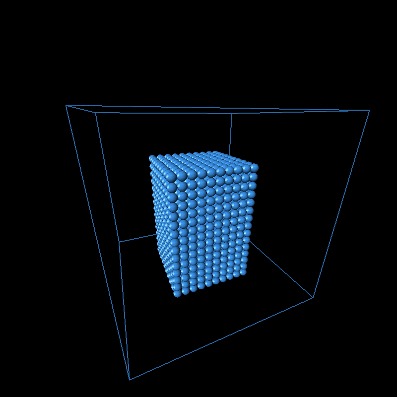
Fluid simulations, at the current time, mostly use algorithms like the Smoothed Particle Hydrodynamics (SPH) that are computationally expensive. In our project, we implement an algorithm belonging to the Position Based Dynamics framework, that takes a particle-driven approach to the simulation of fluids as outlined in the paper of Macklin and Müller. More specifically, we implemented the fluid as a collection of particles subject to incompressibility constraints and separately update the position of these particles after accounting for vorticity confinement and viscosity. In the end, we created animations of a body of fluid that appeared realistic without needing to resort to small intervals of the time step.

Technical Approach

Fluid simulations are frequently utilized in various applications of computer graphics like films and computer games. In real-time applications like computer games, it is important that the images render quickly and this requires that the fluid simulation algorithms be efficient.

The basic strategy of our simulation (based on the algorithm outlined in a paper by Macklin and Müller) is as follows: we model the incompressibility of fluid by a set of nonlinear constraints, one for each particle. These constraints say that the estimate of the density of the fluid at each particle should be equal to some fixed rest density. Specifically, if R_i idenotes the density estimate at particle i and R_0 denotes the rest density then constraint i is given by C_i(p1, ..., pn) = R_i/R_0 - 1. At each time step, we try to find an arrangement of the particles such that all these constraints are 0, using Newton’s method to solve the constraints (so we move the particles in the direction of the gradient of the constraints, approximating the constraints with the first two terms of their Taylor expansions about their current positions). We also use a density estimator to approximate the density of the fluid by the positions of a finite number of particles. We use the density estimators given in the paper, namely the so-called poly6 and spiky kernels (commonly used in SPH simulations). This technique mainly differs from other common techniques in that when we solve the constraints we directly update the positions of the particles, rather than their velocities.

This technique works reasonably well, but introduces a number of problems. One of the main problems is that if a particle is in an area of low density (such as the boundary of the fluid), it will rush towards the other particles in an attempt to satisfy the density constraints. This creates weird looking clumping effects. One interesting way to fix this is to add “ghost particles” around the boundary of the fluid at each step of the constraint solver (these particles contribute to the density estimates but are not altered by the constraint solver and are not rendered). We did not use that approach (but it is a cool idea). Instead, we followed the example of the Macklin and Müller paper and added an artificial pressure term to the position updates (in the constraint solving loop) that pushed particles apart a little bit. However, when this term was too large, it could create surface-tension like effects that also look weird if they are too pronounced.

Another problem that SPH methods have in general is a tendency to lose energy over time. To fix this we added vorticity confinement (another common technique in SPH simulations). Basically, vorticity confinement increases the velocity of particles, but does so in the direction that the fluid was already moving in. Since vorticity confinement requires the calculation of a gradient with no easy analytic form, we found the numerical gradient. Namely, if f(p) is some scalar-valued function that we want to compute the gradient of then one way to do so numerically is to approximate

∇_x f(p) =  (f(p +  d*x) - f(p))/d 

where x indicates the unit vector in the x-direction and d is some small constant. Before the vorticity confinement was added, the fluid had a tendency to quickly settle into an equilibrium, which looks unrealistic. After it was added, the fluid looked a lot more energetic and dynamic.

We also added a viscosity correction to prevent the fluid particles from flying apart too quickly (basically the viscosity correction slows down particles that are near each other and moving in opposite directions).

We added walls around the fluid so it would have something to slosh around in, and we varied the position of one of the walls over time to create waves (which looks a little cooler than just a single splash and then settling to equilibrium).

We also tried implementing a grid acceleration structure (where at the beginning of the constraint solving loop, each particle is hashed to a grid and when calculating the density estimate at a particle, only the particles in its neighboring grid cells are used). However, this did not seem to give a noticeable speed-up. Another optimization we tried was to cache values of the density estimators and use these without recomputing them until the particle positions changed again.

To recap, the basic structure of the program is as follows. For each time step, first update the velocities and positions of the particles based on external forces (in this case, just gravity) and update the position of the moving wall. Then use Newton’s method to move the particle positions to satisfy the density constraints. During the constraint solving loop, add an artificial pressure term to the position updates along with another small correction term. Also, if any particle’s position is moved through a wall, move the particle back inside. After the constraint solving loop is done, update the particle velocities based on the new particle positions and then update the velocities based on the vorticity confinement and viscosity corrections. Repeat for as many time steps as you have patience for. Below is an image of the pseudocode from the paper on Position based Fluids.

Pseudocode of the algorithm implemented


One of the main challenges of this implementation was that there were many parameters (number of steps of Newton’s method, gravity, rest density, smoothing radius for the density estimators, and the various parameters used in calculating artificial pressure, vorticity confinement and viscosity) that control the behavior of the simulation, and tuning them is important to get a good looking fluid. In particular, it can be hard to tell if the program has a bug or you just need to alter the parameters.

One problem we encountered was that early on, the particles had a tendency to fly apart. It turned out that this could be fixed by dividing the particle position updates by the number of neighbors within the smoothing radius of the particle (the smoothing radius controls which particles contribute to the density estimate at a position). This idea was based on a comment by Müller in a tutorial on fluid simulations.

Another problem we had to consider was the exact way in which we were going to implement collision detection. Initially, if we detected that a given particle had gone beyond the wall, we would simply reflect it about the normal of the wall. However, we realized that this was not giving us accurate results and instead decided to update the position of the particle to the point of collision because the reflected position became inaccurate with further updates to its position.

We learned how to use position-based dynamics to approximate the actual dynamics of fluid and how to fix the various problems introduced by this framework. We also learned how important it is to choose good parameters and that when water is compressed it explodes (or at least that simulated water is compressed, it explodes).

Results

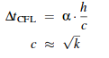
We will compare the efficiency of our algorithm to that of the Smoothed-particle Hydrodynamics (SPH) algorithm. The SPH algorithm, a widely used computational method for simulating fluid flows, adheres to the time step limit imposed by the Courant-Friedrichs-Lewy (CFL) condition shown below. In the equation below, h is the global support radius, c is the velocity of sound propogation in the fluid (related to stiffness), k is the stiffness constant and alpha is just a constant.

Courant-Friedrichs-Lewy (CFL) condition

The SPH approach to fluid dynamics relies on a Lagrangian formulation of fluid dynamics and the CFL guarantees the convergence of the partial differential equations in this formulation (Navier-Stokes' equation). Though we do not have our own version of the SPH solver implemented, due to time constraints, we will use the data collected and presented in a paper on Time Adaptive Approximation SPH as a baseline for comparison of our time step. In this paper, the authors used the SPH but varied the value of the time step based on the number of iterations and the velocity of the moving particle. Based on the graphs of data and algorithm presented in the paper, the highest value of time step they use is 0.012*2.5 = 0.03 s. The value of time step we use is approximately an order of magnitude larger than the highest value used in an improved version of the SPH solver.

After much tweaking, we settled on the following final parameters.

Number of iterations of position update: 5
Rest density: 550 particles per unit volume (mass assumed to be 1)
Time step: 0.1
Smoothing radius: 0.4 (the size of the box was around 1.0)
Gravity (external forces): 0.1

Our final animations, which were made to be gifs, had a time interval of 90 milliseconds between each image. Thus, we ended up with a frame rate of 11 frames per second. Some of the gifs we rendered are shown below.


The simulation below had 4500 particles.
Computer Man


The simulation below had 1500 particles.
Computer Man


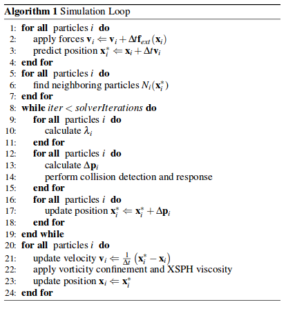
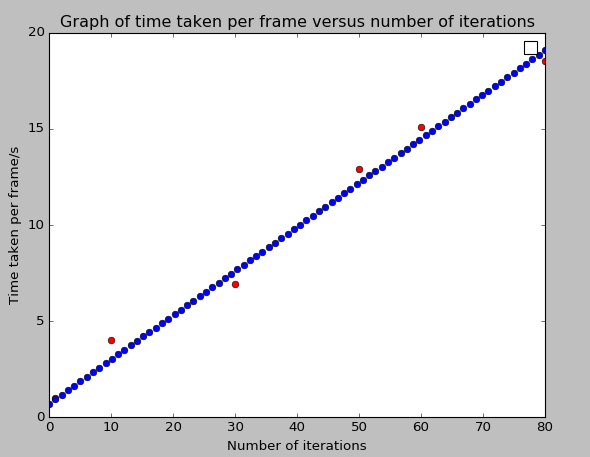
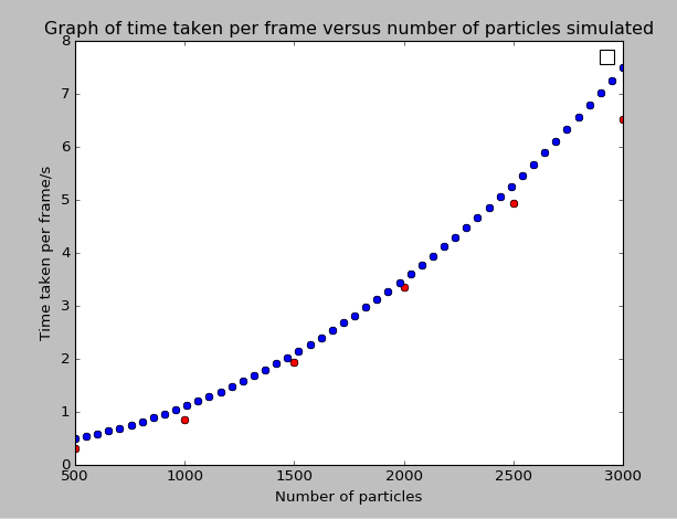
Based on the structure of the algorithm, the runtime increased linearly with the number of iterations and polynomially with the number of particles we were modelling. The iterations in point refer to the iterations of the position update within each frame. The position updates are necessary so that the final image rendered reflects the accurately the positions of the particle. We found that the images generally converged to an accurate one at 5 iterations. An image of the pseudocode is shown at the bottom. This can be seen in the graphs below.


The red data points closely match the blue linear graph


The red data points closely match the blue quadratic y = kx^2 graph

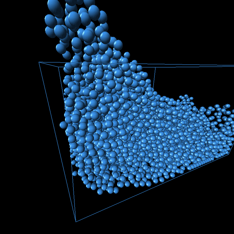
On top of generating the intended animations, we thought it would be fun to play around with the different parameters. The animations of each along with the parameter varied are shown below.


1) The following gif is with 1 iteration. You can see that there is a lot of clumping and violation of rest density constraints. If more iterations were allowed, it would have updated correctly.

Computer Man


2) The following gif is with a low rest density. It behaves somewhat like a gas.

Computer Man


3) The following gif is with a low value of the smoothing radius for the kernel enforcing incompressibility constraints. It is well-behaved initially because the radius is small and particles are far apart enough. Once they get close enough though, the particles go crazy trying to fulfill the constraints.

Computer Man


4) The following gif is with a low value of gravity. The cube of water forms into a sphere (most stable configuration) before falling and even after it falls, it doesn't really flow because of the comparatively higher viscosity.

Computer Man


5) The following gif is with a large time step of 1. The animation loses a lot of its finer details. For instance, the splash isn't quite as dramatic because the time over which the position updates are much longer and hence, several intermediat movements are not captured.

Computer Man


References

1. Lagrangian Fluid Dynamics Using Smoothed Particle Hydrodynamics by Micky Kelager, January 9 2006
2. Position Based Dynamics by Muller et. al, Journal of Visual Communication and Image Representation, April 2007
3. Position Based Fluids by Miles Macklin and Matthias Muller
4. Simulating Gaseous Fluids with Low and High Speeds by Yue Gao et. al, Pacific Graphics 2009
5. Time Adaptve Approximate SPH by Prashant Goswami and Renato Pajarola, VRIPHYS 2011

Contributions from each team member

Patrick Lutz
1. Implemented viscosity
2. Implemented incompressibility constraints (find_lambda, kernel functions etc)
3. Wrote final report and plan for final project
4. Implemented vorticity
5. Generated animations for the animation with larger number of particles and fine-tuned the parameters


Leah Tom
1. Implemented collision detection
2. Implemented vorticity in parallel
3. Wrote final report and plan for final project
4. Implemented moving wall
5. Generated animations with different values of parameters for smaller number of particles

Credits